1. INTRODUCTION
In the past decades, advance in the field of nanophotonics is enough to provoke the onset of the analysis of optical thin films; they are adopted in many optical devices. By investigating numerous optical properties of nanophotonic structures, obtained responses facilitate an extended realm of applications: Electrodes in a lithium-ion battery [1], solar control coating [2], optically switchable thin films [3-5], optical filters [6], and Bragg reflectors [7-9]. Especially, thin films contribute to most fields, from nanophotonics, material science, and even biomedical disciplines [10,11].
Along with the drastic growth of computer science, exceptional computational algorithms are proposed, simply solving the Maxwell equations repetitively. This concept, however, turned out to be computationally expensive and lacks efficiency in that electromagnetic simulation entails a numerous number of calculations: Rigorous coupled-wave analysis (RCWA) [12,13], finite difference time domain (FDTD) [14], finite element method (FEM) [15], transfer-matrix method (TMM) [16], and scattering- matrix method (SMM) [17,18].
Besides the conventional methods, deep learning (DL) has contrived to take account of its high-throughput nature [19]. This unprecedented approach can effectively handle a sizeable amount of data with ease. Since a deep neural network (DNN) learns the generalized pattern of the given data set, the quality and size of the set is a pivotal concern. Considering its promising prediction capability, which is trained using backpropagation and non-linear activation functions [20] to address the “black-box” method, DNN derives a generalized function to approximate the pattern, which implies a relationship between input and output of the data set. In this manner, the model simply mimics Maxwell's equations, not by intuitively knowing the mathematical computation process, but by the accumulated sense acquired through training. As a one-off cost process, the results can be promptly retrieved once the model is trained.
The promising characteristic of DL empowers almost every field to implement the state-of-the-art algorithm over outdated ones: Image analysis in medical fields [21], DL-based inspection systems for the smart factory [22], and so on. To keep up with the move, we propose and implement a basic structure of DNN to derive optical spectral responses of multilayered optical thin films. In this work, we exploit several adjustable features to carry out an analysis and comparison of the performance of the model. By juxtaposing the tendency of the cost function, which is mean squared error (MSE), it is expected that each variable is optimized: 1) number of layers, 2) model architecture, 3) size of data set, and 4) train, test, validation split ratio.
Notably, under several settings, the model excellently approximates the target response. The affection of each variable is closely examined through the comparison of reflectance spectra with different conditions. According to the simulations, the DNN with five input variables consisting of the four hidden layers with 512-256-256-128 neurons is the most efficient trial among others, while MSE is lowest when the network is fed with the data set of 150,000 unique designs separated into train, test, validation with the ratio of 6:2:2. Although the distinguished setting can be varied as target changes, any other problems can be resolved by tuning the suggested variables.
2. MODELS AND METHODS
Basically, multilayered optical thin films hold three associated features manifesting the optical properties of the design: Reflectance (R), transmittance (T), and absorptance (A). The conservation of energy governs how reflectance, transmittance, and absorptance are interrelated, i.e.,
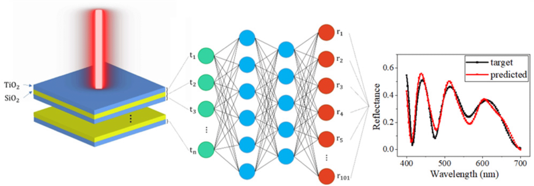
In this study, we have accumulated training data set using algorithm which employed RCWA method. The data gathering algorithm initializes the multilayered thin films with the number of layers ranging from two to five are composed of alternating layers of titanium dioxide (TiO2) and silicon dioxide (SiO2), which are considered as a sample structure for the study. The thickness of each layer is selected randomly in the range of [10, 300] nm, with a 10 nm interval. Also, a total of 101 equally spaced discrete points of the refractive index of TiO2 and SiO2 have sampled in the range of [400, 700] nm. This sample rate is enough to meticulously detect the whole spectrum. Given that the suggesting materials are lossless, which means no absorption (A=0) takes place as the light goes through the material, we calculate only the reflectance of the films; transmittance can be omitted owing to the Eqn. 1 (T=1−R).
In the data preparation phase, the size of training data sets varies from 1,000 to 500,000 taking account of the attributes of each variable (i.e., 1,000 for two layers, 500,000 for five layers). To derive the reflectance spectrum from the suggested design, we opted for RCWA due to its high reliability and fast calculation [23].
In this work, the primary concern is to approximate the Maxwell equations using DNN, so that the trained model can immediately predict the optical spectral response of the suggested design without carefully examining it. Thus, we employed the general DNN with several tunable features, which allow us to figure out the optimal conditions for training. The suggested DNN receives the thickness of each layer as an input while predicting the reflectance as a learning output. The underlying concept is based on polynomial regression due to the curvilinear profile of the spectrum. The developed network involves a loss function, activation function, and optimizer, which are integral to training. Without any change, the elemental level of DNN is fed with 200,000 data separated into training, test, and validation with a ratio of 8:1:1, respectively. Besides, the rectified linear unit (ReLU) [24] is employed as an activation function, while adam optimizer, which spontaneously updates the learning rate, is chosen for its distinguished performance [25]. In the training session, we adopted MSE as a cost function and trained for 200 iterations. The threshold of MSE is defined, referring to the MSE between two reliable simulators using an electro-magnetic concept. The DNN is trained with the training set, and then the validation set is applied to conduct cross-validation for every epoch. The final model, in turn, implies the minimum value of validation loss, so it can be verified using the test set.
With the general DNN, we now allow several variations to the model for a deliberate analysis of each factor; how the result would be changed as a pivotal parameter varies. Typically, factors that are likely to have a meaningful impact on performance are selected as tunable features.
The number of layers varies from two to five, while the amount of data for each step also varies proportionally. For the structure of DNN starts with simple architecture, then proceeds to a relatively deep network. The size of the data set increases gradually from 25,000 to 150,000. Additionally, for the train, test, validation split ratio, the proportion of the train set decreases, while that of the test and validation set increases at an identical rate.
3. RESULTS AND DISCUSSION
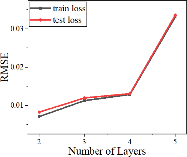
Increasing the number of layers does not merely add more complexity to the design, but the number of combinations (i.e., 302 for two layers, 303 for three layers, considering the potential candidates of a thickness of each layer). Thus, MSE shows an upward trend as the number of layers increases. In Fig. 1, the MSE, which implies the average discrepancy between target and predicted response throughout the whole samples, is relatively low at which the number of layers is lower than five. However, as the number of combinations soars from the five layers, it is quite challenging for the network to reduce the loss to the extent of previous models.
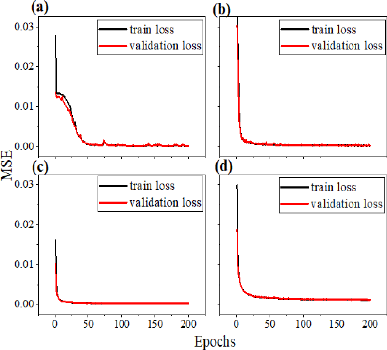
The number of designs in the data set varies since the possible number of combinations is different. The number of structures in each model is 1,000, 30,000, 200,000, and 500,000, respectively. On account of the number of designs varies for each model, the learning curves in Fig. 2 show that the MSE of all four networks converges as the number of training epochs increases.
The inclination of MSE in Fig. 1 implies that the performance of predicting the spectral response tends to cause degradation. As expected, spectrums in Fig. 3 come up with similar results; first to third networks approximate the target response very clearly, while the last model manifests noticeable errors between the two spectra. Through the first analysis, we found that the number of layers more than five might provoke meaningful errors if other features remain the same.
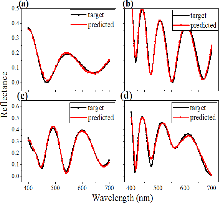
The number of neurons in each hidden layer defines how deep and complicated the network is. Specifically, total parameters play a pivotal role in evaluating the performance of the model. As the number of layers and neurons increases, more and more parameters contribute to figuring out a sophisticated function, which can approximate the delicate features. A trained network with a larger MSE value tends to suggest a rough profile because simple architecture cannot reach the point at which a deeper network can attain.
Table 1 displays the detailed information of each architecture and RMSE value. The change in RMSE seems to be marginal, but even a minute difference between the networks can yield a magnified error in the model evaluation session.
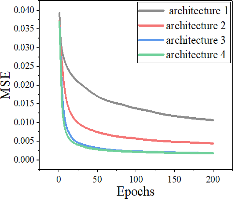
Fig. 4 shows the learning curves of four different architectures. It is clear that the simplest one has the most gradual change in MSE throughout the 200 training iterations, while others express a drastic fall in MSE. All things considered, although there is an additional layer with 1,024 neurons in architecture 4, MSE changed infinitesimally. Accordingly, Fig. 5 corroborates the assumption that the performance and complexity of the network are dependent to a certain extent. Gradual increase in prediction level tends to converge as the total number of parameters of the network exceeds a certain number.
Basically, DL requires a large amount of data set to figure out the internal pattern and relationships. However, if it is too much, it can result in a huge waste of time in data preparation and training processes with marginal benefit obtained. Thus, it is essential to stay within an affordable range.
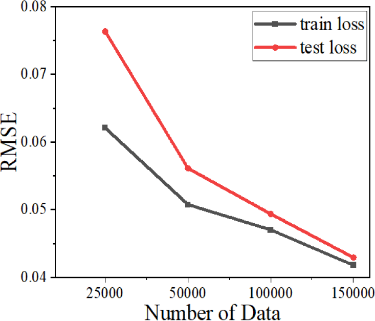
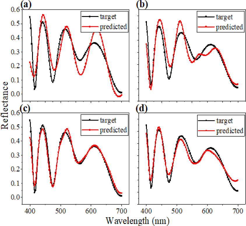
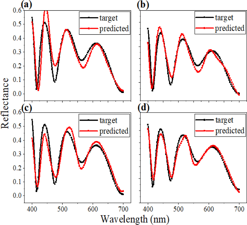
As shown in Fig. 6, a downward trend of MSE supposedly indicates the larger data set gives birth to a discriminating model. However, this can be controversial, taking into account the one-time cost property of DL. Of course, a larger data set contributes to the better performance of the network. Nevertheless, from the point at which the MSE starts converging, there are no more benefits from aggrandizing the size of the data set.
Learning curves in Fig. 7 have a similar profile compared to each other. Although the number of unique structures is almost tripled. Even if the size of the data set matters the most, it becomes a meaningless factor, as it becomes too large to train with. Although Fig. 8 shows an appreciable change in approximation performance, a sizeable data set cannot be regarded as only the right path. For the forward prediction of five layers, all other conditions being considered the same, approximately 200,000 unique designs can derive the internal pattern of the given data set.
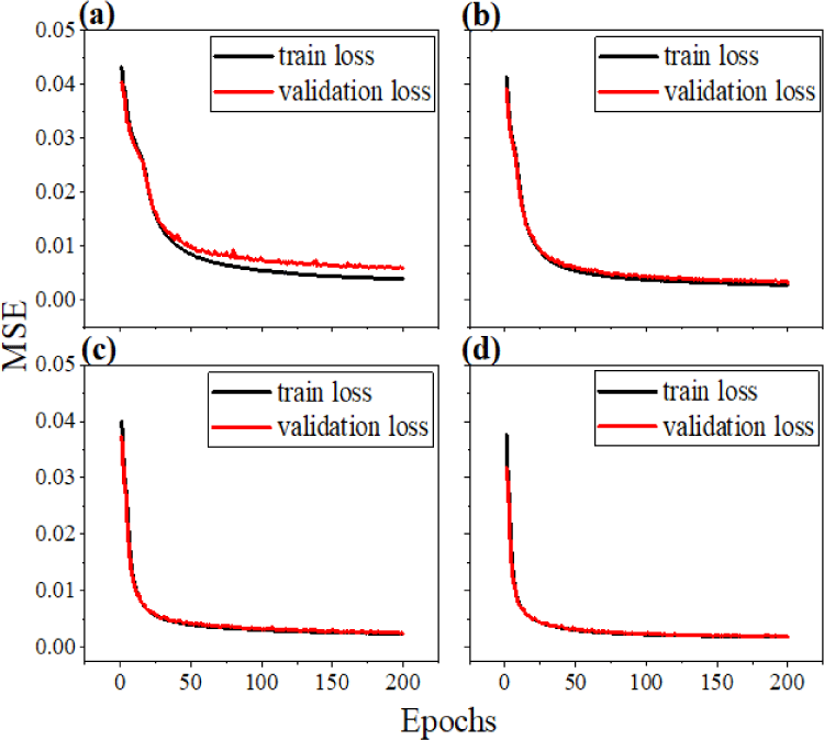
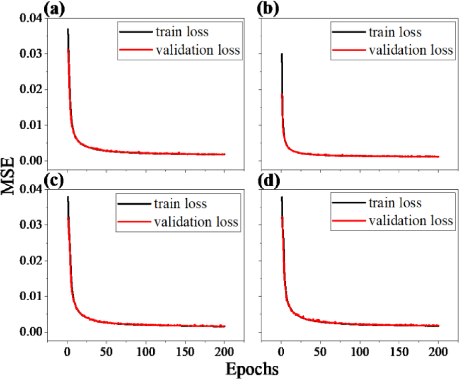
Separation of the given data set into several clusters contributes to enhanced performance as well as reliability. Solely placing the training set for the DL can result in over-fitting, which indicates that the trained network can predict outputs from inputs that have been used in the previous training session. The trained model cannot proceed with the totally unfamiliar data set. To handle the issue, a validation set is employed to prevent the over-fitting problem. Further, to get refined results while training, a test set is also implemented to evaluate the final model. Despite the fact that the adoption of the test and validation set is promising, the optimal ratio of each data set is not defined yet. It varies from case to case. Thus, now we take a look at Fig. 9, which describes the learning curves of four difference ratio models. Even though we noticeably changed the ratio of each data set, there seems to be no difference between them. Similarly, Fig. 10 with four different predictions shows that the model performs the best when the ratio of train, test, and validation is 6:2:2.
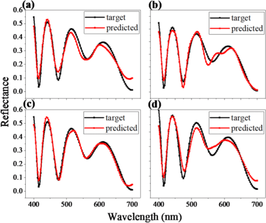
Likewise, the other factors can also be the governing ones, as the fields and applications vary. Considering the underlying characteristics of DL, optimal conditions for one project can have a poor performance on the other one. The impact and influence of variables are closely examined by juxtaposing reflectance spectra with different initial conditions. According to the simulations, the DNN with five input variables composed of the four hidden layers with 512-256-256-128 neurons shows the minimum MSE when the network is fed with the data set of 150,000 unique designs separated into the train, test, validation with the ratio of 6:2:2.
4. CONCLUSION
In conclusion, we have implemented general DNN to predict the spectral response of multilayered optical thin films in lieu of the conventional Maxwell equations. Considering the underlying properties of DL, a rapid calculation based on the pattern identification of the given data set eventually encourages DL to substitute for the existing genetic algorithms. In this work, we first tried to demonstrate the validity of DL as an optimization tool. By suggesting several pivotal variables—1) number of layers, 2) model architecture, 3) size of data set, and 4) train, test, validation split ratio-to be tuned, it is possible to identify the optimal condition for the specific parameter. The MSE tends to soar as the number of layers stacked more than five. Also, using a convergence theory, the optimal network is established, which consists of four hidden layers with 512-256-256-128 neurons in each layer. Further, a total of 150,000 unique sets of designs are fed to the established network, separated into train, test, and validation sets with a ratio of 6:2:2, respectively. Since the presented conditions are confined to fixed circumstances, we expect to conduct further research to relieve the constraints for further development of the fields of nanophotonics.

